The Black-Scholes Option Pricing Model: From Theory to Interactive Application
The Problem
Imagine you pay 10 dollars today for a contract that gives you the right to buy Apple stock at 150 anytime before March 1st. If Apple rises to 180, you exercise your right, buy at 150, and pocket 30 (minus the 10 you paid). If Apple falls to 120, you simply don't exercise; you lose only your initial 10.
This contract is called an option, and a trader holding one faces a deceptively simple question:
What is this option worth today, and how does that value change across hundreds of possible market scenarios?
In this example, the stock the option is based on, Apple, is called the underlying asset. The 150 purchase price locked into the contract is the strike price, and March 1st is the expiration date.
A single price calculation answers none of the questions that matter in practice:
- If the stock drops 10% tomorrow, what happens to my position?
- If the market becomes more uncertain (volatility increases), do I profit or lose?
- How much value will I lose by holding this position for another week?
- Under what combinations of price and uncertainty does my trade become profitable?
The Black-Scholes model, published in 1973, solved the theoretical pricing problem and earned its creators a Nobel Prize (Black, Scholes, 1973; Merton, 1973). Yet the model's output, a single number, leaves traders without answers to the questions above. In this post, I'll walk through the complete theoretical framework, implement it in Python, and extend it through interactive visualization to bridge the gap between theory and practical decision-making.
1. The Nature of Options
Why Do Options Exist?
Options are like insurance for stocks. Just as you pay a premium for car insurance that protects you from losses, you pay a premium for an option that either protects your downside or lets you profit from upside, depending on the type.
There are two basic types:
- Call option: The right to buy the stock at a fixed price. You profit if the stock rises above that price.
- Put option: The right to sell the stock at a fixed price. You profit if the stock falls below that price.
The key word is right, not obligation. If the market moves against you, you simply walk away and lose only what you paid for the option.
A Concrete Example
Suppose a stock trades at 100 today. You buy a call option with:
- Strike price (
): 105 (the price at which you can buy) - Expiration (
): 30 days from now - Premium paid: 3
Scenario 1: Stock rises to 120. You exercise, buy at 105, and sell at 120. Profit: 120 - 105 - 3 = 12.
Scenario 2: Stock falls to 90. You don't exercise (why buy at 105 when it trades at 90?). Loss: 3 (your premium).
This asymmetry of unlimited upside with capped downside is what makes options valuable and why pricing them correctly is hard.
The Payoff Formula
At expiration, the math is simple. Take whichever is larger: the profit from exercising, or zero (if exercising would lose money):
where is the stock price at expiration, and is the strike price.
In our example: if and , then Call Payoff = .
European vs. American Options
One distinction matters: European options can only be exercised at expiration, while American options can be exercised anytime before. The Black-Scholes model prices European options. American options require more complex methods, though for calls on non-dividend-paying stocks, the prices are identical (it's never optimal to exercise early).
The Pricing Problem
We know what the option is worth at expiration: the payoff formulas above. The hard question: what should we pay today for this uncertain future payoff?
This is the problem Black and Scholes solved.
2. Modeling Stock Price Dynamics
To price an option, we need to model how stock prices move over time. This section builds from intuition to the mathematical model.
The Random Walk Analogy
Imagine a person walking along a number line. Each second, they flip a coin:
- Heads: step right (+1)
- Tails: step left (-1)
After many steps, where will they be? We can't predict exactly, but we can describe the probability distribution of outcomes. This is a random walk.
Stock prices behave similarly: unpredictable moment-to-moment, but with patterns we can model statistically.
Two Key Properties of Stock Prices
Property 1: Percentage moves, not dollar moves
A 100 stock and a 10 stock might both move "a lot" in a day. But "5" means very different things:
- 100 → 105 is a 5% gain
- 10 → 15 is a 50% gain
Stock returns are better described as percentages. Mathematically, this means we model multiplicative changes, not additive ones.
Property 2: Prices can't go negative
A stock can drop 50%, then another 50% (now at 25% of original), then another 50% (12.5%)... but it never hits zero or goes negative. The percentage model handles this naturally.
Drift and Volatility
Two parameters describe how a stock moves:
-
Drift (
): The average direction. Think of a slight hill, where our random walker tends to drift uphill over time. For stocks, this reflects long-term growth. -
Volatility (
): How erratic the movements are. Low volatility = steady progress. High volatility = wild swings. A stock with 20% annual volatility might swing ±20% in a typical year.
Geometric Brownian Motion (GBM)
Combining these ideas mathematically gives us Geometric Brownian Motion:
Don't let this intimidate you. It says:
The tiny change in stock price (
) equals:
- A drift component:
(the stock drifts at rate)- A random component:
(random shocks scaled by volatility)
The term represents the randomness. Technically it's called a "Wiener process," but you can think of it as a continuous coin flip that adds unpredictable noise.
Why "Geometric"? Because changes are proportional to current price ( appears on the right side). A 100 stock is twice as volatile in dollar terms as a 50 stock with the same .
The Key Mathematical Result
From the model above, we can derive where the stock price will be at time . The logarithm of the future price follows a normal distribution:
Translation: Future stock prices are log-normally distributed. They can go up a lot, but can't go below zero.
The here refers to the normal distribution, the familiar bell curve. We'll use this distribution heavily in the Black-Scholes formula, where gives the probability that a standard normal variable is less than .
How Realistic Is This Model?
The GBM model has known limitations. Real stock returns show:
-
Fat tails: Extreme moves (crashes, spikes) happen more often than GBM predicts. The 1987 crash was a 25-standard-deviation event under GBM, essentially impossible under the model's assumptions, yet it happened.
-
Volatility clustering: Calm periods and chaotic periods tend to cluster, but GBM assumes constant volatility.
Dhesi et al. (2019) found that Student-t distributions fit stock data better than the normal distribution GBM assumes. Mandelbrot (1963) and Fama (1965) documented these issues decades ago.
Despite these limitations, GBM remains the foundation of derivatives pricing. It's "wrong but useful": simple enough to yield closed-form solutions while capturing the essential behavior. More realistic models like stochastic volatility (Heston, 1993) and jump-diffusion (Merton, 1976) build on this foundation.
3. Risk-Neutral Valuation
This section explains the core insight that makes option pricing possible. It's subtle, but understanding it demystifies the entire Black-Scholes approach.
The No-Arbitrage Principle
Arbitrage means "free money," profit without risk. Example: if Apple stock trades at 150 on NYSE and 151 on London, you buy on NYSE and sell in London. Free 1 per share.
Markets eliminate arbitrage quickly. If free money exists, traders exploit it until prices align. This simple observation, the no free lunch principle, is the foundation of all derivatives pricing.
The Replication Insight
Here's the key idea: if we can build a portfolio of stocks and bonds that produces the exact same payoff as an option in every possible scenario, then the option must cost exactly what the portfolio costs.
Why? If the option cost more, you'd sell the option and buy the portfolio for the same payoff, but you pocket the difference. If the option cost less, you'd buy the option and sell the portfolio. Either way, free money. Markets don't allow this.
A Concrete Example
Consider a simplified world where a 100 stock can only go to 120 (up) or 80 (down) after one period. We want to price a call option with strike 100.
Option payoffs:
- If stock = 120: Call pays 120 - 100 = 20
- If stock = 80: Call pays 0 (worthless)
Can we replicate this with stocks and bonds?
Suppose we buy shares and borrow dollars. Our portfolio value:
- If stock =
120\Delta - B(1+r)$ - If stock =
80\Delta - B(1+r)$
Setting these equal to option payoffs:
Solving: (buy half a share),
The replicating portfolio costs:
This must be the option price. No model assumptions required, just no-arbitrage logic.
The Risk-Neutral Shortcut
The replication argument works but requires solving portfolio weights for each option. Black and Scholes found a shortcut: we can skip replication and directly compute the expected payoff, if we pretend investors don't care about risk.
In this "risk-neutral world":
- Everyone is indifferent between risky and safe investments
- Therefore, all assets must earn the risk-free rate
on average - We replace the real drift
with
This isn't saying investors actually ignore risk. It's a mathematical trick: the replication argument forces option prices to behave as if investors were risk-neutral, even though they're not.
The Pricing Formula
Under the risk-neutral measure, the option price equals the discounted expected payoff:
Where:
discounts future value to present value (a dollar tomorrow is worth less than a dollar today)means "expected value in the risk-neutral world"is what the option pays at expiration
The stock price dynamics become:
Notice: (real-world drift) is gone, replaced by (risk-free rate). The volatility stays the same.
The Formal Foundation
This risk-neutral pricing framework rests on the Fundamental Theorem of Asset Pricing, formalized by Harrison and Kreps (1979). The theorem proves that no-arbitrage conditions guarantee the existence of a risk-neutral measure under which our pricing formula holds.
The math is deep, involving measure theory and martingales, but the intuition is simple: replication forces a unique price, and risk-neutral pricing computes that price efficiently.
Practical note: You don't need to understand measure theory to use Black-Scholes. Just accept this as a validated shortcut: "pretend everyone is risk-neutral, discount at the risk-free rate, and you get the correct arbitrage-free price." It works.
4. The Black-Scholes Formula
We now have all the pieces: a model for stock prices (GBM) and a pricing principle (risk-neutral expectation). Evaluating the expected payoff gives us the famous Black-Scholes formula.
The Formula
where:
What Does Each Part Mean?
Before memorizing the formula, understand what it's saying:
The function: This is the cumulative normal distribution, which converts a number into a probability between 0 and 1. If you've seen a bell curve, tells you "what percentage of the distribution lies below ."
For a call option, :
| Term | Meaning |
|---|---|
| Expected stock value if exercised, weighted by probability |
| Strike price, discounted to present value |
| Probability the option finishes "in the money" (worth exercising) |
Intuitively: "What I'll receive if I exercise" minus "What I'll pay if I exercise."
The and terms measure how far "in" or "out" of the money the option is, adjusted for time and volatility. Think of them as "standardized moneyness," measuring how many standard deviations away from the strike.
A Quick Sanity Check
When the stock price is very high relative to strike ():
andbecome large positive numbers- Formula becomes
, so the option is worth roughly "stock minus discounted strike"
When the stock price is very low ():
andbecome large negative numbers, so the option is nearly worthless
This matches intuition: deep in-the-money options behave like stock; deep out-of-the-money options are nearly worthless.
Implementation
The formula translates directly into code:
def call_price(S: float, K: float, T: float, r: float, sigma: float) -> float:
    d1 = (np.log(S / K) + (r + 0.5 * sigma ** 2) * T) / (sigma * np.sqrt(T))
    d2 = d1 - sigma * np.sqrt(T)
    return S * norm.cdf(d1) - K * np.exp(-r * T) * norm.cdf(d2)
Where norm.cdf is the cumulative normal distribution from scipy.stats.
5. The Greeks: Quantifying Risk
The Black-Scholes formula gives a single price. But traders need to understand sensitivity: how does the price change when inputs change?
The Greeks answer these "what if" questions. They're called Greeks because they're named after Greek letters, except Vega, which isn't actually a Greek letter but follows the naming convention.
The Five Key Greeks
| Greek | Formula | Question Answered |
|---|---|---|
Delta ( | | How much does my option move per $1 stock move? |
Gamma ( | | How fast does delta change? |
Vega ( | | How sensitive am I to volatility changes? |
Theta ( | | How much value do I lose per day? |
Rho ( | | How sensitive am I to interest rate changes? |
Here is the cumulative normal distribution from Section 4, and is the normal density, the bell curve itself. While gives the area under the curve up to , gives the height of the curve at .
Intuition for Each Greek
-
Delta: If delta = 0.6, the option moves 0.60 for every 1 the stock moves. Calls have positive delta (0 to 1); puts have negative delta (-1 to 0).
-
Gamma: Delta isn't constant; it changes as the stock moves. Gamma measures this rate of change. High gamma means delta swings rapidly.
-
Vega: Options gain value when volatility rises because there's more chance of big moves. Vega measures this sensitivity. A vega of 0.15 means a 1% increase in volatility adds 0.15 to the option price.
-
Theta: Time decay. Options lose value as expiration approaches because there's less time for favorable moves. Theta is typically negative, so each day costs you money.
-
Rho: Interest rate sensitivity. Usually small and often ignored in practice.
Implementation
def delta(S, K, T, r, sigma, option_type):
    d1 = (np.log(S / K) + (r + 0.5 * sigma ** 2) * T) / (sigma * np.sqrt(T))
    return norm.cdf(d1) if option_type == 'call' else norm.cdf(d1) - 1

def gamma(S, K, T, r, sigma):
    d1 = (np.log(S / K) + (r + 0.5 * sigma ** 2) * T) / (sigma * np.sqrt(T))
    return norm.pdf(d1) / (S * sigma * np.sqrt(T))

def theta(S, K, T, r, sigma, option_type):
    d1 = (np.log(S / K) + (r + 0.5 * sigma ** 2) * T) / (sigma * np.sqrt(T))
    d2 = d1 - sigma * np.sqrt(T)
    term1 = -(S * norm.pdf(d1) * sigma) / (2 * np.sqrt(T))
    if option_type == 'call':
        return (term1 - r * K * np.exp(-r * T) * norm.cdf(d2)) / 365
    return (term1 + r * K * np.exp(-r * T) * norm.cdf(-d2)) / 365
The Theta-Gamma Tradeoff
A fundamental relationship connects these sensitivities. Options that profit from big moves (high gamma) necessarily suffer more time decay (negative theta). You can't have one without the other.
At-the-money options (where stock price = strike price) have the highest gamma and the most negative theta. This makes intuitive sense: these options are on the knife's edge, most sensitive to which way the stock moves, but also most vulnerable to time running out.
Mathematically, the Black-Scholes PDE implies:
For at-the-money options with low interest rates, this simplifies to:
Translation: owning gamma costs theta. This tradeoff is inescapable; it's built into the mathematics.
6. Beyond Single Points: The Visualization Problem
A single option price tells a trader nothing about risk. The Greeks provide local sensitivities, but traders need to understand the entire landscape of possible outcomes.
Consider a trader who purchased a call option for $10.45. The relevant questions are:
- At what stock price does the position break even?
- How does this breakeven shift if volatility changes?
- What region of the price-volatility space produces profits versus losses?
Answering these questions requires computing option values across a grid of scenarios, potentially thousands of calculations.
Vectorized Grid Computation
NumPy enables efficient evaluation across parameter grids:
def calculate_option_grid(S_base, K, T, r, sigma_base, n_steps=50):
    stock_prices = np.linspace(S_base * 0.8, S_base * 1.2, n_steps)
    volatilities = np.linspace(sigma_base * 0.5, sigma_base * 1.5, n_steps)
    S_grid, sigma_grid = np.meshgrid(stock_prices, volatilities, indexing='ij')

    d1 = (np.log(S_grid / K) + (r + 0.5 * sigma_grid**2) * T) / (sigma_grid * np.sqrt(T))
    d2 = d1 - sigma_grid * np.sqrt(T)

    calls = S_grid * norm.cdf(d1) - K * np.exp(-r * T) * norm.cdf(d2)
    puts = K * np.exp(-r * T) * norm.cdf(-d2) - S_grid * norm.cdf(-d1)
    return calls, puts, stock_prices, volatilities
This computes 2,500 option prices in a single vectorized operation.
7. Interactive Heat Maps
Heat maps transform numerical grids into visual insight. I used Plotly for interactive exploration:
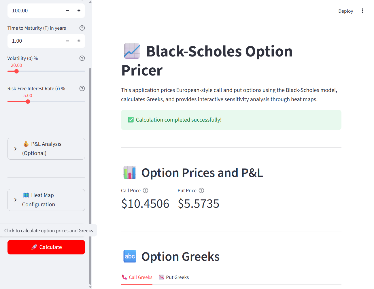
Figure 1: The application displays computed option prices and Greeks with interactive visualization.
The call value heat map reveals how option value increases with stock price (horizontal axis) and volatility (vertical axis). Warmer colors indicate higher values.
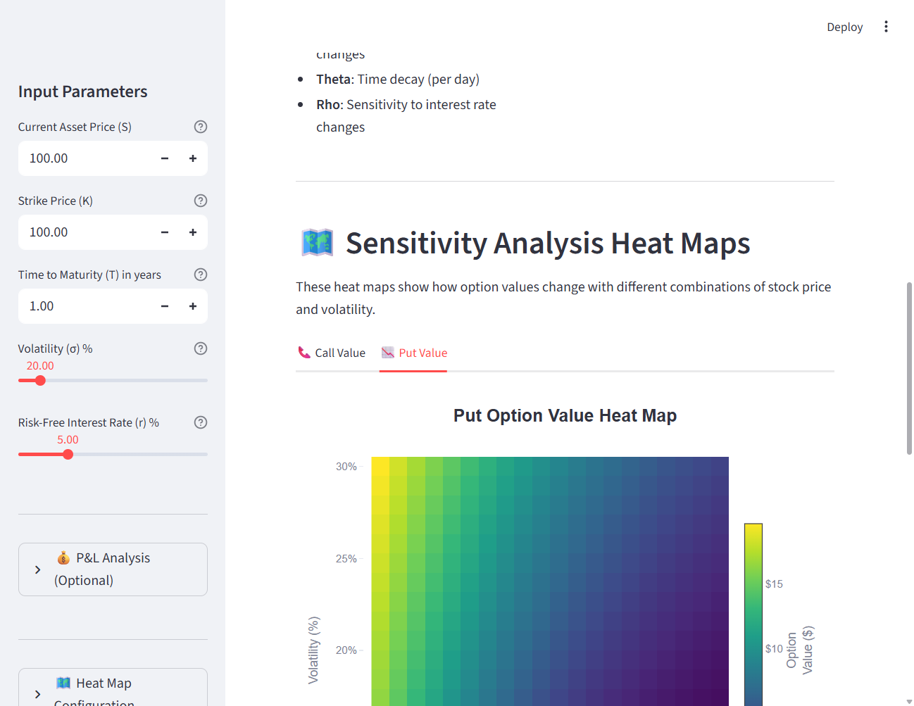
Figure 2: Put option values show the inverse relationship: value increases as stock price decreases.
P&L Visualization
For traders with existing positions, the critical visualization is profit and loss:
def create_pnl_heatmap(data, stock_prices, volatilities):
    max_abs = max(abs(data.min()), abs(data.max()))
    fig = go.Figure(data=go.Heatmap(
        z=data.values,
        x=stock_prices,
        y=volatilities * 100,
        colorscale='RdYlGn',
        zmid=0,
        zmin=-max_abs,
        zmax=max_abs
    ))
    return fig
The diverging red-green colorscale, centered at zero, immediately distinguishes profitable scenarios (green) from losing scenarios (red).
Heat maps show us the landscape of prices we calculate, but in practice we often observe market prices and need to work backwards. This leads to a critical question: what volatility is the market assuming?
8. Implied Volatility
So far, we've used Black-Scholes to compute price from volatility. In practice, the question often reverses: given an observed market price, what volatility does the market imply?
The Reverse Problem
Think of it like a recipe in reverse. You see a cake priced at 20 and know the recipe (Black-Scholes formula). You can work backwards to figure out how much the baker is charging for eggs (volatility).
Implied volatility (IV) is the volatility value that, when plugged into Black-Scholes, produces the observed market price. It tells you how much uncertainty the market is pricing in.
Why care about IV?
- Compare options: A call with IV of 40% is pricing in more uncertainty than one with IV of 20%
- Forecast expectations: High IV before earnings = market expects big moves
- Identify mispricings: If your volatility estimate differs from IV, you might have a trading opportunity
The Numerical Challenge
Unlike forward pricing, there's no formula to directly compute IV. We must solve:
"Find
such that BS-Price() = Market Price"
This requires iterative numerical methods.
Newton-Raphson Method
The Newton-Raphson algorithm iteratively improves our volatility guess:
Translation: adjust the guess proportionally to how wrong we are, scaled by vega (how sensitive price is to volatility).
Convergence is rapid when vega is large (Quant Next, 2023). However, deep out-of-the-money options (where strike is far from current price) have near-zero vega, causing numerical instability. Robust implementations use bisection search as a fallback.
def implied_volatility(price, S, K, T, r, option_type, tol=1e-6):
    sigma = 0.5
    for _ in range(100):
        bs_price = call_price(S, K, T, r, sigma) if option_type == 'call' else put_price(S, K, T, r, sigma)
        diff = bs_price - price
        if abs(diff) < tol:
            return sigma
        d1 = (np.log(S / K) + (r + 0.5 * sigma**2) * T) / (sigma * np.sqrt(T))
        vega = S * norm.pdf(d1) * np.sqrt(T)
        if vega < 1e-10:
            raise ValueError("Vega too small")
        sigma -= diff / vega
        sigma = max(sigma, 0.01)
    raise ValueError("Failed to converge")
9. Model Limitations
Before relying on Black-Scholes in practice, you must understand where it fails. The model rests on assumptions that don't hold in real markets:
-
Constant volatility: Real volatility varies over time and across strikes, producing the "volatility smile" (Dupire, 1994).
-
Log-normal returns: Real return distributions exhibit fat tails and excess kurtosis.
-
Continuous trading: Transaction costs make continuous rebalancing impossible.
-
No jumps: Extreme events occur more frequently than GBM predicts. The 1987 crash was a 25-standard-deviation event under the model, effectively impossible.
Despite these limitations, Black-Scholes remains the industry standard. It's widely used as a practical approximation while traders understand its constraints.
10. The Complete Application
I built an interactive web application that integrates pricing, Greeks, and visualization:
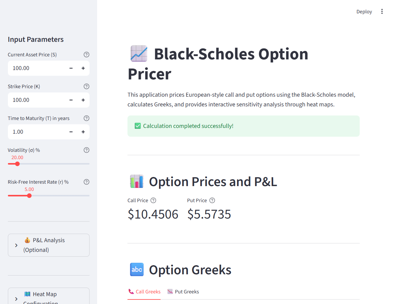
Figure 3: The complete application with input parameters, computed values, and heat maps.
Users input parameters through the sidebar, click Calculate, and immediately see:
- Option prices for calls and puts
- All five Greeks with visual representation
- Interactive heat maps across price and volatility scenarios
- P&L analysis when purchase prices are provided
- Export capabilities for further analysis
The app also persists calculations to SQLite for historical comparison.
Conclusion: Answering the Question
We began with a question: What is this option worth, and how does that change across possible futures?
The Black-Scholes model provides the theoretical foundation: a closed-form solution derived from no-arbitrage arguments and risk-neutral valuation. The Greeks quantify local sensitivities. But neither addresses the trader's need to understand the full landscape of outcomes.
The implementation I built bridges this gap. Remember the four questions from the opening?
| Question | Answer |
|---|---|
| "If the stock drops 10% tomorrow, what happens to my position?" | Delta tells you the immediate impact; heat maps show the full range |
| "If volatility increases, do I profit or lose?" | Vega quantifies sensitivity; heat maps visualize all volatility scenarios |
| "How much value will I lose by holding another week?" | Theta gives daily decay rate |
| "Under what combinations does my trade become profitable?" | P&L heat maps show the exact profit/loss boundary |
The complete system maps theory to practice:
| Component | Problem Solved |
|---|---|
| Pricing engine | Fair value calculation |
| Greeks functions | Local sensitivity measurement |
| Vectorized grid computation | Efficient scenario analysis |
| Heat map visualization | Intuitive understanding of the price-volatility surface |
| P&L coloring | Immediate identification of profitable vs. losing scenarios |
| Persistent storage | Historical comparison and audit |
The mathematical elegance of Black-Scholes translates into working software. The software, through visualization, transforms abstract sensitivities into intuitive understanding. A trader can now see (not just calculate) how their position responds to market movements.
This represents the proper relationship between theory and practice: rigorous mathematics provides the foundation, implementation makes it operational, and visualization makes it useful.